Introduction
This document is an attempt at explaining different types of fractals and techniques to create beautiful renderings.
First we start by explaining what shaders are and how you can program them in GLSL. Then we will do a quick refresh on the math that is required for complex numbers. If you think that math is not your thing, the functions to do the complex arithmetic in GLSL are implemented in this document and you can simply copy them. However, after the Mandelbrot section there is no more escaping from the math, and basic knowledge of algebra, vectors, and matrices will help tremendously.
Armed with the knowledge of basic GLSL programming and complex numbers, we will start to render the Mandelbrot set. The core ideas of rendering fractals are explained here. When we have a rendering of the set, we will explore a technique for coloring. The coloring technique is developed by Iniqo Quilez, and I think it is so simple and powerful that any programmer can benefit from it. To complete the rendering program, we will also implement supersampling. With supersampling we are 'measuring' multiple points in the pixel and average them out to get the final color. This gives an anti-aliasing effect, where jagged edges become more smooth (less pixelized look).
Shaders and GLSL
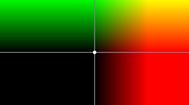
Example Shader
void mainImage( out vec4 fragColor, in vec2 fragCoord )
{
    // Normalized pixel coordinates (from 0 to 1)
    vec2 R = iResolution.xy;
    vec2 uv = (2.*fragCoord - R) / R.y;

    // color as a vector of 3 components: red, green, blue.
    vec3 col = vec3(uv.x, uv.y, 0.);

    // draw crosshair
    if(abs(uv.x) < 0.01 || abs(uv.y) < 0.01) col = vec3(.5);

    // draw circle
    if(dot(uv, uv) < 0.001) col = vec3(1);

    // Output to screen
    fragColor = vec4(col,1.0);
}
Random Numbers
float random (in vec2 st) {
    return fract(sin(dot(st.xy, vec2(12.989,78.233))) * 43758.543);
}

float rseed = 0.;
vec2 random2() {
    vec2 seed = vec2(rseed++, rseed++);
    return vec2(random(seed + 0.342), random(seed + 0.756));
}
Complex Numbers
A complex number $z$ is defined as a a number with two components, indicating that they are two dimensional. An example is $z=3+2i$, which can be generalized to $z=a + bi$. In a complex number, $a$ is called the real component, and $b$ is called the imaginary component. Like normal arithmetic, the rules for addition and multiplication have been defined for complex numbers. However, for complex numbers the arithmetic is differently from what you are used to do with real numbers. How to do the arithmetic with complex numbers is explained in a later section. Another notation that is used in complex numbers is $\textrm{Re}(z)$ to refer to the real component, and $\textrm{Im}(z)$ to refer to the imaginary component. This means that a complex numbers can also be written as $z=\textrm{Re}(z) + i\ \textrm{Im}(z)$.
Open a Python REPL, and define a complex number with
complex(a, b). This is an easy way to play with complex arithmetic.
Geometric Interpretation of Complex Numbers
Another way to think about complex numbers, is with $x$ and $y$ coordinates. In this idea the real component is the $x$ value, and the imaginary component is the $y$ value. For example, $z=3+2i$ can be plotted on the complex plane:
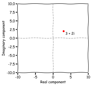
This gives us a nice way to think about complex numbers. Namely, a complex number can be thought of as a point in the $xy$-plane.
Rules of Complex Arithmetic
Complex arithmetic is defined a bit differently from what you are used to do with real numbers, because they are two dimensional. If have have two complex numbers $a + bi$ and $c + di$, then:
- Addition: $(a + bi) + (c + di) = a + c + i(b + d)$.
- Example: $(3 + 2i) + (1 - i) = 4 + i$.
- Multiplication: $(a + bi)(c + di) = ac + adi + bci + bdi^2 = ac - bd + i(ad + bc)$, notice that $i^2 = -1$, thus $bdi^2 = - bd$.
- Example: $(3 + 2i)(1 - i) = 3 - 3i + 2i - 2i^2 = 5 - i$.
- Exponentiation: $(a + bi)^2 = a^2 + 2abi + b^2i^2 = a^2 - b^2 + 2abi$.
- Example: $(3 + 2i)^2 = 9 + 6i + 6i + 4i^2 = 5 + 12i$.
Open a Python REPL and verify the examples to get a feel for it. It's easier than you think.
Complex Arithmetic in GLSL
In GLSL we represent complex numbers with a vector of two components. If we can encode the complex arithmetic in terms of matrix operations, the calculations can be accelerated by the hardware of the GPU. In this section, we will derive these matrix operations. For example, if we have two complex numbers $a + bi$ and $c + di$, we can write this the vectors $u = [a, b]$ and $v = [c, d]$.
Addition
The first case we will consider is addition. It can be achieved trivially with vector addition. Both components will be added to each other. Thus to add them the operation simply is $u+v$.
Multiplication
The second case is multiplication. First we create a matrix $A = \begin{bmatrix} a && b \\ -b && a \end{bmatrix}$ from the vector $u$. For the complex multiplication of $u\cdot v$, we replace $u$ with the matrix $A$. When we work out the matrix multiplication:
$$ A\cdot v = \begin{bmatrix} a && b \\ -b && a \end{bmatrix} \cdot \begin{bmatrix}c \\ d \end{bmatrix} = \begin{bmatrix} ac-bd \\ ad+bc \end{bmatrix},$$the result is the same as the multiplication rule: $(a + bi)(c + di) = ac - bd + i(ad + bc)$.
Exponentiation
The last case is exponentation. The case $u\cdot u$ is a simplified version of the multiplication case, since we can just multiply the complex number by itself. Here we replace the first $u$ with $A$, and work out $A\cdot u$ to get:
$$ A\cdot u = \begin{bmatrix} a && b \\ -b && a \end{bmatrix} \cdot \begin{bmatrix}a \\ b \end{bmatrix} = \begin{bmatrix} a^2-b^2 \\ 2ab \end{bmatrix},$$which is the same as the exponentiation rule: $(a + bi)^2 = a^2 - b^2 + 2abi$.
Implementation
The implementation in GLSL of the operations follows easily from the formulas.
u + v                  // addition       u+v (vector addition)
mat2(u, -u.y, u.x) * v // multiplication u*v (matrix multiplication)
mat2(u, -u.y, u.x) * u // exponentiation u^2 (matrix multiplication)
The Mandelbrot Set
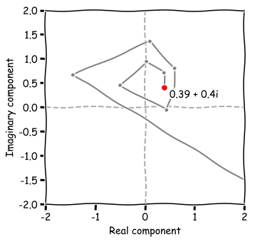
Pick a complex number $c$, for example $c = 0.3 + 0.1i$, and $z = 0 + 0i$. For the first iteration we calculate $z^2 + c$, which is $(0 + 0i)^2 + 0.3 + 0.1i = 0.3 + 0.1i$. For the second iteration we set $z = 0.3+0.1i$, and then we find that $z^2 + c = 0.38 + 0.16i$. If we repeat this proces and plot the points we get after each iteration:
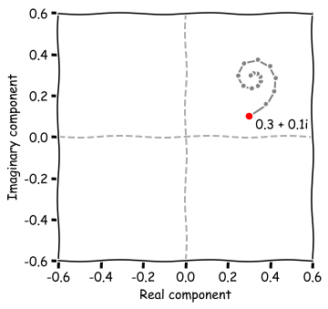
As we can see the points are spiraling inwards to a point. The path that the complex number takes when iterating is called the orbit. It is clear that the orbit is converging towards a point. The other case is that the orbit quickly grows after each iteration and soon shoots off to infinity.
If the point shoots to infinity, the point is not in the Mandelbrot set. We can check this while iterating and it happens when $|z| > B$. Based on how fast the point shoots to infinity, and how many iterations we are doing, a color is determined. We divide the iterations $i$ by the number of iterations $N$, to get a value between $[0, 1]$. This scalar value is used to map to a color. If the point stayed within the bounds $B$ during all iterations, it is in the Mandelbrot set and we color it black.
The proces we described above is perfectly suited for the GPU. Each pixel on the screen, can be mapped, as an example to the range of $[-2, 2]$ on the complex plane, and then we follow the orbit of that complex number when we iterate with the Mandelbrot formula.
The Mandelbrot set is given with:
$$ z_{n+1} = z_n^2 + c $$Clasically we pick a bound $B=2$ which is the disk that contains the Mandelbrot set. To remove this disc, we increase $B$ to $4$ or higher. On each iteration we calculate $z = z^2 + c$, and check if $|z|$ is greater than $B$, meaning that the orbit of $z$ will escape to infinity. This happens when $\sqrt{a^2 + b^2} > B$, which we can square to get $a^2 + b^2 > B^2$. The next thing we can do is to rewrite $a^2 + b^2$ as the dot product $z\cdot z$. This leads to the following equation that we can use to check if $z$ has escaped to infinity: $z\cdot z > B^2$. Rewriting it algebraically removes the necessity of the square root operation, which improves the speed of the algorithm.
The following GLSL code is a simple and fast implementation for rendering the Mandelbrot set.
#define N 64.
#define B 4.

void mainImage( out vec4 fragColor, in vec2 fragCoord ) {

    vec2 R = iResolution.xy;
    vec2 uv = (2. * fragCoord - R - 1.) / R.y;
    vec2 z = vec2(0), c = uv;
    float i;

    for(i=0.; i < N; i++) {
        z = mat2(z, -z.y, z.x) * z + c;
        if(dot(z, z) > B*B) break;
    }

    if(i==N) { i = 0.; } // mark interior black
    fragColor = vec4(vec3(i/N), 1.);
}
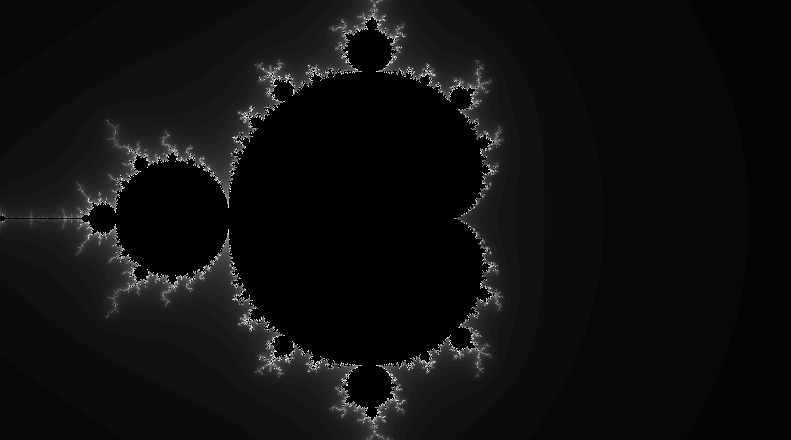
It will render the following image:
The code can be refactored a little bit by moving iteration into a new function iterate(float p). We can also scale the image by multiplying uv by $1.2$. Finally, to center the image we subtract $[0.4, 0.0]$ from uv. This results in the final code for this section:
#define N 64.
#define B 4.

float iterate(vec2 p) {
    vec2 z = vec2(0), c = p;
    float i;
    for(i=0.; i < N; i++) {
        z = mat2(z, -z.y, z.x) * z + c;
        if(dot(z, z) > B*B) break;
    }
    return i;
}

void mainImage( out vec4 fragColor, in vec2 fragCoord ) {

    vec2 R = iResolution.xy;
    vec2 uv = 1.2 * (2. * fragCoord - R - 1.) / R.y - vec2(.4, 0.);

    float n = iterate(uv) / N;
    if(n==1.) n = 0.;
    fragColor = vec4(vec3(n), 1.0);
}
The end result should look like this:

So far we have created the Mandelbrot itself, but the white coloring is quite boring. In the next section we will explore a technique which allows us to create color gradients with a surprisingly simple formula.
Colorful Palettes
When we calculated the Mandelbrot set, we apply colorization based on the value of $n$, which has been normalized between $[0,1]$. The idea in this chapter is to develop a function with a parameter $t$ ranging between $[0,1]$, that returns a color from a gradient. The gradient can be composed out of many different colors, also called a palette.
Procedural Color Palette
A simple way to create a procedural color palette has been created by Inoqo Quilez) , it is the following cosine expression:
As $t$ runs from $0$ to $1$, the cosine oscillates $c$ times with a phase of $d$. The result is scaled and biased by $a$ and $b$ to meet the desired contrast and brightness. The parameters $a, b, c$ and $d$ are vectors with three components (r, g, b). We can also think of $a$ as the offset, $b$ as the amplitude, $c$ as the frequency, and $d$ as the phase, for each r, g, b component respectively.
For example, if we pick values for $a, b, c$ and $d$:
we can create a plot with the cosine gradient generator. This gives a nice visualization of what is going on and how this procedural color palette works.
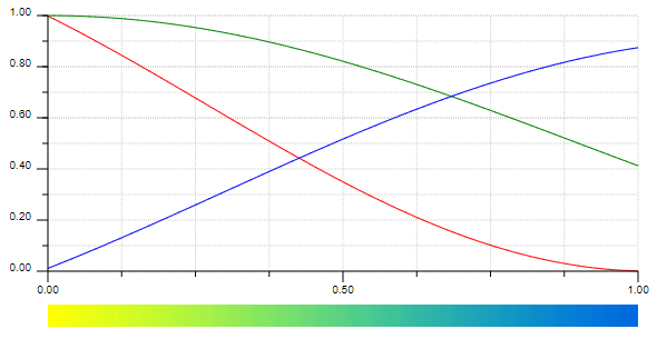
We can see that each of the r, g, b components sits on a cosine wave and they are mixed together with sliding $t$ between $[0,1]$. This set of values gives a nice yellow, green and blueish gradient.
Gradient Examples
This section contains a table with different palettes that can be used as a color map.
| a | b | c | d | palette |
|---|---|---|---|---|
[0. 0.5 0.5] |
[0. 0.5 0.5] |
[0. 0.5 0.33] |
[0. 0.5 0.66] |
 |
[0.938 0.328 0.718] |
[0.659 0.438 0.328] |
[0.388 0.388 0.296] |
[2.538 2.478 0.168] |
 |
[0.66 0.56 0.68] |
[0.718 0.438 0.72 ] |
[0.52 0.8 0.52] |
[-0.43 -0.397 -0.083] |
 |
[0.5 0.5 0.5] |
[0.5 0.5 0.5] |
[0.8 0.8 0.5] |
[0. 0.2 0.5] |
 |
[0.821 0.328 0.242] |
[0.659 0.481 0.896] |
[0.612 0.34 0.296] |
[ 2.82 3.026 -0.273] |
 |
[0.5 0.5 0.5] |
[0.5 0.5 0.5] |
[1. 1. 1.] |
[0. 0.33 0.67] |
 |
[0.5 0.5 0.5] |
[0.5 0.5 0.5] |
[1. 1. 1.] |
[0. 0.1 0.2] |
 |
[0.5 0.5 0.5] |
[0.5 0.5 0.5] |
[1. 1. 1.] |
[0.3 0.2 0.2] |
 |
[0.5 0.5 0.5] |
[0.5 0.5 0.5] |
[1. 1. 1.] |
[0.8 0.9 0.3] |
 |
[0.5 0.5 0.5] |
[0.5 0.5 0.5] |
[1. 0.7 0.4] |
[0. 0.15 0.2 ] |
 |
[0.5 0.5 0.5] |
[0.5 0.5 0.5] |
[2. 1. 0.] |
[0.5 0.2 0.25] |
 |
[0.5 0.5 0.5] |
[0.5 0.5 0.5] |
[2. 1. 1.] |
[0. 0.25 0.25] |
 |
This is a list of palettes have been created by http://dev.thi.ng/gradients, and Iniqo Quilez. More gradients can be created with http://dev.thi.ng/gradients.
Implementation
The code follows easily from the formula described above:
vec3 palette( in float t, in vec3 a, in vec3 b, in vec3 c, in vec3 d )
{
    return a + b*cos( 6.28318*(c*t+d) );
}
Smooth Iteration Count
As you probably have noticed, the change in color goes in discrete steps, which creates the color bands. This happens because $n$, the number of iterations, is an integer. These discrete steps of changes in colors results in the rendering of the bands. To solve this problem, Iniqo Quilez explains a method that determines the fractional part of $n$. We subtract the fractional part from $n$ to get $sn$, which is smooth.
The fractional part of the smooth iteration count can be calculated with:
where $B$ is the threshold when $|z|$ has escaped, and $d$ is the degree of the polynomial under iteration. In the case where $d=2$, such as in the Mandelbrot set, an optimized variant is available:
Implementing the non-optimized version can be done by having the line in the iterate function:
return i;
perform the formula we described above, which in GLSL is:
return i - log(log(dot(z, z)) / log(B)) / log(2.);
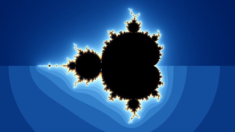
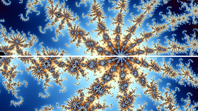
The next image is a rendering of a comparison between both methods. The smooth iteration count can be seen in the top part of the rendering, and the integer iteration count in the bottom half.
#define N 64.
#define B 4.

vec3 pal( in float t, in vec3 a, in vec3 b, in vec3 c, in vec3 d ) {
    return a + b*cos( 6.28318*(c*t+d) );
}

float iterate(vec2 p) {

    vec2 z = vec2(0), c = p;
    float i;

    for(i=0.; i < N; i++) {
        z = mat2(z, -z.y, z.x) * z + c;
        if(dot(z, z) > B*B) break;
    }

    if(p.y < 0.) return i;
    return i - log(log(dot(z, z)) / log(B)) / log(2.);;
}

void mainImage( out vec4 fragColor, in vec2 fragCoord ) {

    vec2 R = iResolution.xy;
    vec2 uv = 1.2 * (2. * fragCoord - R - 1.) / R.y - vec2(.4, 0.);
    float sn = iterate(uv) / N;

    vec3 col = pal(fract(sn + 0.5), vec3(.5), vec3(.5),
                   vec3(1), vec3(.0, .1, .2));

    fragColor = vec4(sn == 1. ? vec3(0) : col, 1.0);
}
Supersampling
When we calculate the color at the position of a pixel, this position is an integer value. For example, if the resolution of your screen is $1920\times1080$, we can pick a point $(500, 500)$. The next pixel would be at $(501, 500)$. The idea of supersampling is, instead of finding the color once, to find the color multiple times at different offsets and calculate the average. This average will become the final color of the pixel.
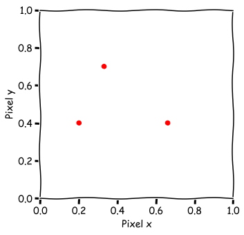
Instead of finding the color at $(500, 500)$, we pick three other points, such as:
- $(500.28, 500.64)$
- $(500.78, 500.33)$
- $(500.11, 500.87)$
This is simply the point, and we have added a random value between $[0, 1]$ to the $x$ and $y$ position.
For each of those points we will find the color with the iterate function. To find the final color, take the sum of all the colors we have found, and divide this by the amount of points we tested.
#define N 1024.
#define B 256.
#define SS 16.

float random (in vec2 st) {
    return fract(sin(dot(st.xy, vec2(12.989,78.233))) * 43758.543);
}

float rseed = 0.;
vec2 random2() {
    vec2 seed = vec2(rseed++, rseed++);
    return vec2(random(seed + 0.342), random(seed + 0.756));
}

vec3 pal( in float t, in vec3 a, in vec3 b, in vec3 c, in vec3 d ) {
    return a + b*cos(6.28318 * (c*t + d));
}

float iterate(vec2 p) {

    vec2 z = vec2(0), c = p;
    float i;

    for(i=0.; i < N; i++) {
        z = mat2(z, -z.y, z.x) * z + c;
        if(dot(z, z) > B*B) break;
    }

    return i - log(log(dot(z, z)) / log(B)) / log(2.);;
}

void mainImage( out vec4 fragColor, in vec2 fragCoord ) {

    vec2 R = iResolution.xy;

    vec3 col = vec3(0);
    for(float i=0.; i < SS; i++) {

        vec2 uv = 0.001 * (2. * fragCoord + random2() - R) / R.y
            - vec2(.892, -0.23527);

        float sn = iterate(uv) / N;

        col += pal(fract(6.*sn), vec3(.5), vec3(0.5),
                   vec3(1.0,1.0,1.0), vec3(.0, .10, .2));
    }

    fragColor = vec4(col / SS, 1.0);
}
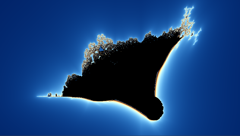
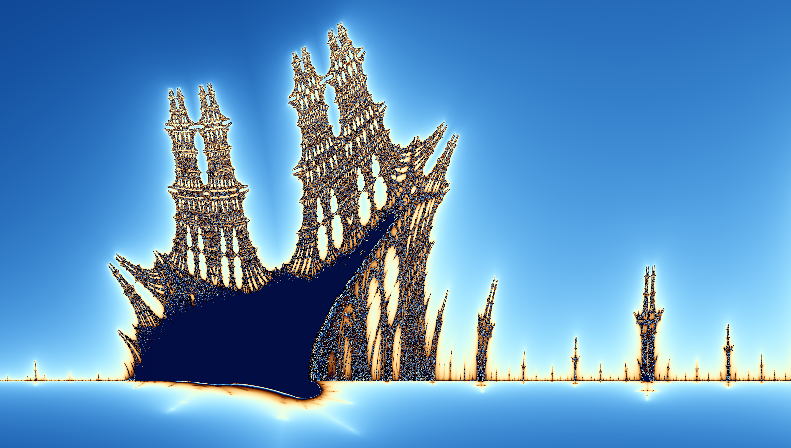
Burning Ship Fractal
vec2 uv = 0.05 * (2. * fragCoord + random2(R+i) - R) / R.y - vec2(1.73, -0.035);
#define N 64.
#define B 32.
#define SS 4.

float random (in vec2 st) {
    return fract(sin(dot(st.xy, vec2(12454.1,78345.2))) * 43758.5);
}

vec2 random2(in vec2 st) {
    return vec2(random(st), random(st));
}

vec3 pal( in float t, in vec3 a, in vec3 b, in vec3 c, in vec3 d ) {
    return a + b*cos(6.28318 * (c*t + d));
}

float iterate(vec2 p) {

    vec2 z = vec2(0), c = p;
    float i;

    for(i=0.; i < N; i++) {
        z = abs(z);
        z = mat2(z, -z.y, z.x) * z + c;
        if(dot(z, z) > B*B) break;
    }

    return i - log(log(dot(z, z)) / log(B)) / log(2.);;
}

void mainImage( out vec4 fragColor, in vec2 fragCoord ) {

    vec2 R = iResolution.xy;

    vec3 col = vec3(0);
    for(float i=0.; i < SS; i++) {

        vec2 uv = 1.3 * (2. * fragCoord + random2(R+i) - R) / R.y
            - vec2(0.4, -0.55);

        uv.y = -uv.y;

        float sn = iterate(uv) / N;

        col += pal(fract(2.*sn + 0.5), vec3(.5), vec3(0.5),
                   vec3(1.0,1.0,1.0), vec3(.0, .10, .2));
    }

    fragColor = vec4(col / SS, 1.0);
}
Julia Sets
Animation
Rotation over time
Zoom over time
Polynomials